Prerequisites

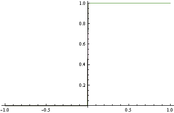
True data generating process p(y=1|x)

In[39]:=

Out[40]=

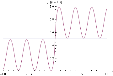
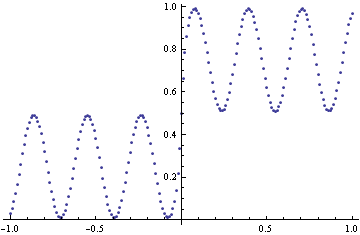
To make optimization tractable, compute loss by summing losses over the following points

In[3]:=

Out[4]=

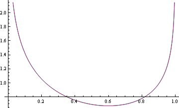
Define log - loss and truncated log loss. Truncated log loss is used to avoid numerical problems (getting Log[1/0] during optimization). Using truncated loss has an effect that once the function gets close to 1 or 0, getting it closer no longer decreases the loss.

In[5]:=

Out[7]=

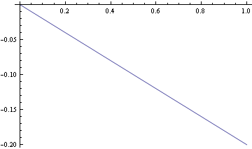
Linear/hinge loss. In this case we are considering probability models that never go outside of (0, 1) Since hinge loss and linear loss are identical over that domain, use linear loss

In[8]:=

Out[9]=

In[10]:=

Out[11]=

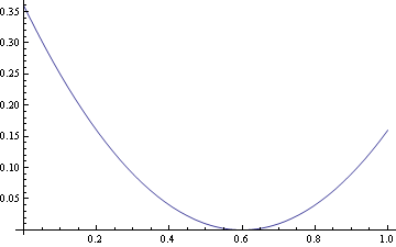
Fitter

In[12]:=

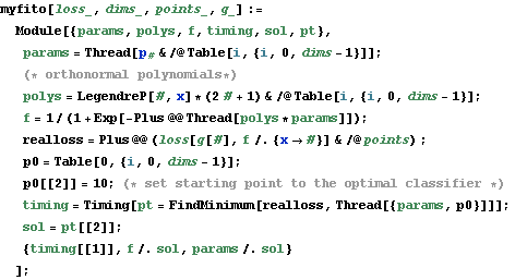
Best fit using log - loss and 2 degrees of freedom corresponds to Bayes optimal classifier

In[13]:=

Out[14]=

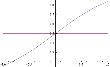
Because some points are on the boundary (g (x) = 1), and our function class does not include those points, there may not be a minimum, however, because we initialize the starting value to function that produces the optimal classifier, we can be sure that the result of minimization gives better loss than the starting point (it might be equal in the case of the Hessian being 0, which is not the case here). You can see that with higher degree of freedom you can decrease log loss, but that increases 0-1 loss.

In[15]:=

Out[16]=

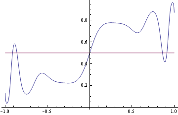
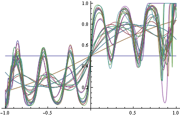
Find minimizers values for all degrees of from 2 to 30. There are warnings, likely due to the fact that minimum is outside of the achievable region (step function is not achievable exactly)

In[220]:=

Out[220]=

In[90]:=

Out[90]=

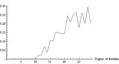
Evaluate approximation error

In[203]:=

In[204]:=

Out[204]=

In[205]:=

Out[205]=

In[207]:=

Out[207]=

Created by Wolfram Mathematica 6.0  (12 June 2007)